Taguchi Dynamic-Standardized Analysis

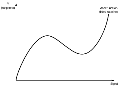
The nonlinear relation illustrated in the following figure is not easily modeled by traditional dynamic $S / N$ ratio formulations of zero point proportional form, reference point proportional, or the general linear equation form.

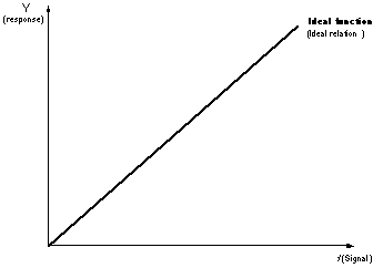
With the new dynamic-standardized analysis approach, measurement spaces are transformed into linear spaces and are analyzed using methods similar to the traditional dynamic analysis approach.

The procedure employed in this new approach is a two-step approach, as shown below. Conceptually, the procedure is similar to traditional Taguchi approaches:

Step 1 - Maximize Robustness (Minimize Variation)
One goal with Taguchi methods is to always reduce the response variation caused by the affects of uncontrollable noise. Control factor settings are sought that minimize the effects of the noise factors.
Step 2 – Adjust System Behavior to Target
In this case the “mean on target” Taguchi goal is actually expanded by the requirement to move the entire signal-response relationship to the “ideal” or target relationship.

Step 1. Maximize robustness

Step 2. Adjust system behavior to target

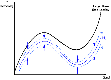
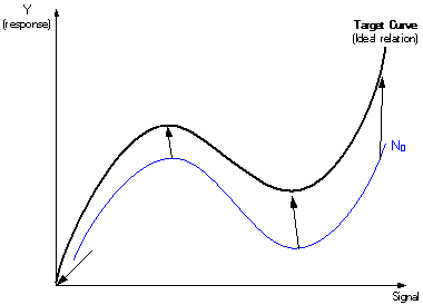
The processes illustrated in the figures above are performed in the transformed “linearized” space. In the new measurement space, the $Y$ values of the reference noise condition are plotted on the X-axis and the observed response values are plotted on the Y-axis. The reference noise condition is user-specified. It can be defined by a certain noise condition or by a hypothetical zero-noise condition. As a result of the transformation, the curve of $N_{0}$ , the reference noise condition, becomes a line through the origin and at a $45 °$ angle with the X-axis, as shown in the following figure.

The curves of the other noise conditions $N_{1}, N_{2}$ will vary around the $N_{0}$ reference noise condition, not necessarily linearly.

The transformed measurement space can be analyzed effectively by means of traditional dynamic analysis of the zero point proportional $S / N$ ratio. However, the new $S / N$ ratio in the linearized space is not identical to the traditional $S / N$ ratio, because in the linearized space, $β$ in $y = β M$ is expected to be constant value of 1. (The $β$ can take arbitrary values in the traditional dynamic $S / N$ ratio formulation.)

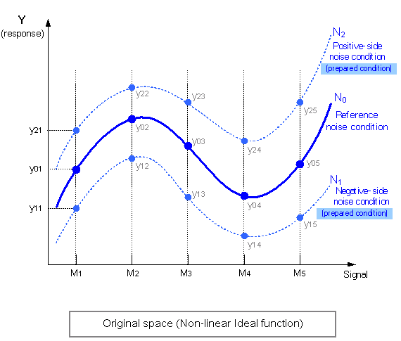
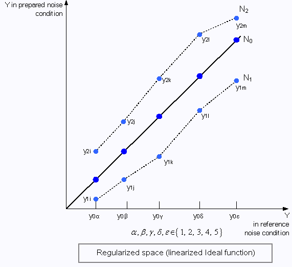
Transformation of Measurement Space

		$M_{1},$	$M_{2},$	$\dots,$	$M_{k}$
Reference noise condition	$N_{0}$	$y_{01}$	$y_{02}$	$\dots,$	$y_{0 k}$
Negative-side prepared noise condition	$N_{1}$	$y_{11}$	$y_{12}$	$\dots,$	$y_{1 k}$
Positive-side prepared noise condition	$N_{2}$	$y_{21}$	$y_{22}$	$\dots,$	$y_{2 k}$

In the dynamic-standardized approach, the use of three noise conditions as previously discussed (reference noise condition, negative-side noise condition, and positive-side noise condition) is recommended over the use of a full noise matrix to reduce calculation effort. For nonlinear problems, more signal levels are needed to represent this nonlinearity than traditionally used with dynamic analysis (often two or three signal levels are used with traditional dynamic analysis; four or more is common with the new dynamic-standardized approach). The total calculation effort is the product of the control matrix times the noise matrix times the number of signal levels. The use of three noise conditions instead of a full noise matrix can offset the added computational cost with the increase in the number of signal levels.

The three noise conditions $(N_{0}, N_{1}, a n d N_{2})$ are user defined. The combinations of noise factor levels necessary to define $N_{0}, N_{1}, a n d N_{2}$ are generated in one of two ways:

specified manually, based on user knowledge, or
through preprocessing experimentation—running a separate noise experiment, identifying main effects of the noise factors, and choosing appropriate levels for each for the negative side and positive side.

If a full noise matrix is employed, a reference noise condition is still employed. This reference noise condition is often estimated using the average response values at each signal level. This approach allows for application of the dynamic-standardized $S / N$ methodology.

The dynamic-standardized analysis employs a standardized $S / N$ ratio formulation. Two versions of this $S / N$ ratio formulation can be employed. Both versions are available in Isight and are shown below:

Standardized $S / N$ ratio (generic version):
Standardized $S / N$ ratio (Taguchi version):

where
$r$ is the sum of the squares of the reference response values
$S_{β}$ is the variation caused by the proportional effect
$V_{e}$ is the pure error variance
$V_{N}$ is the noise error variance

The denominator in the generic version is divided by $1 / 2 r$ . This step is different from the traditional definitions of $S / N$ ratio.

Once the standardized $S / N$ ratio values are calculated for all control experiments, the calculated main effects can be used to “tune” the design for robustness and to adjust the system behavior to the target “ideal” conditions. A transformation concept similar to that used for the dynamic-standardized $S / N$ ratio approach is employed for this tuning. The values of the X-axis in this transformation are the target response values (the reference response targets) under $N_{0}$ for each signal level. The values of the Y-axis are calculated response values. Combinations of control factor levels can then be explored to achieve a linear relationship in this transformed measurement space.

This tuning, illustrated in the figure below, is shown in the following procedure:

Step 1: Estimate the $y$ curve in the polynomial expression: $y = β_{1} m + β_{2} m^{2} + β_{2} m 3$ . The polynomial expression is based on orthogonal expansion.
Step 2: Find a combination of control factor levels to achieve $β_{1} - > 1, β_{2} - > 0, β_{3} - > 0$ .

The polynomial is calculated for each row of the control matrix.

	$M_{1},$	$M_{2},$	$\dots,$	$M_{k}$
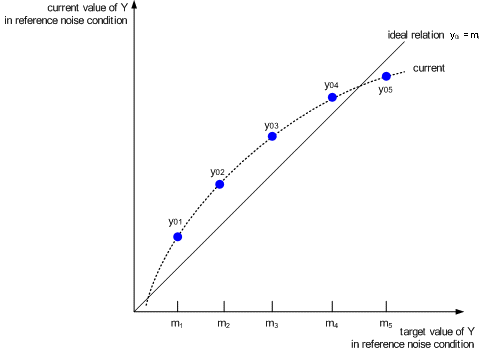
Target value (reference noise condition)	$m_{1}$	$m_{2}$	$\dots,$	$m_{k}$
Response value (reference noise condition)	$y_{01}$	$y_{02}$	$\dots,$	$y_{0 k}$

With the dynamic-standardized analysis approach, as with traditional Taguchi approaches, the calculated main effects are used to tune the design. The main effects of the control factors on the standardized $S / N$ ratio are used to achieve robustness. The main effects of the control factors on the $β_{1}, β_{2} a n d β_{3}$ are used to adjust system behavior to the target condition.