RBF and EBF Models

Overview

Radial Basis Functions (RBF) are a type of neural network employing a hidden layer of radial units and an output layer of linear units. Elliptical Basis Functions (EBF) are similar to Radial Basis Functions but use elliptical units in place of radial units. Compared to RBF networks where all inputs are handled equally, EBF networks treat each input separately using individual weights.

RBF networks are characterized by reasonably fast training and reasonably compact networks. On the other hand, EBF networks require more iterations to learn individual input weights and are often more accurate than RBFs.

Weissinger (1947) was the first to use numeric potential flow to calculate the flow around wings. The potential flow equations are a radial basis function. Hardy (1971) realized that the same concept could be used to fit geophysical data to geophysical phenomena. Broomhead and Lowe (1988) renamed this technology “neural nets,” and it was subsequently used to approximate all types of behavior.

An advantage of choosing EBF over RBF is EBF’s ability to rank the input variables in the order of influence on the output variables as described in Ranking the Influence of Input Variables on Output Variables.

Usage in Isight

Isight follows the Hardy (1972, 1990) method as described by Kansa (1999).

Let $x_{1}, \dots, x_{N} \in Ω \subset R^{N}$ be a given set of nodes. Let $g_{i} (x) \equiv g (‖ x - x_{j} ‖) \in R, j = 1, \dots, N$ , be a set of any radial basis functions. Here $‖ x - x_{j} ‖$ is the Euclidian distance given by ${(x - x_{j})}^{T} (x - x_{j})$ . Given interpolation values $y_{1}, \dots, y_{N} \in R$ at data locations $x_{1}, \dots, x_{N} \in Ω \subset R^{N}$ , RBF interpolant

\begin{matrix} (1) & F (x) = \sum_{j = 1}^{N} α_{j} g_{j} (x) + α_{N + 1} \end{matrix}

is obtained by solving the system of $N + 1$ linear equations

\begin{matrix} (2) & \sum_{j = 1}^{N} α_{j} g_{j} (x_{i}) + α_{N + 1} = y_{i}, i = 1, \dots, N \end{matrix}

\begin{matrix} (3) & \sum_{j = 1}^{N} α_{j} = 0 \end{matrix}

for $N + 1$ unknown expansion coefficients $α_{j}$ .

Hardy (1972, 1990), the primary innovator of the RBF Method, adds a constant to the expansion and constraints the sum of the expansion coefficients to zero as seen in Eqn 1 and Eqn 2, introducing the notation

p = [\begin{matrix} 1 \\ ⋮ \\ 1 \end{matrix}] \in ℜ^{N}, G = [\begin{matrix} {\begin{matrix} g \end{matrix}}_{1} (x_{1}) & \dots & g_{N} (x_{1}) \\ ⋮ & ⋮ & ⋮ \\ g_{N} (x_{1}) & \dots & g_{N} (x_{N}) \end{matrix}] \in ℜ^{N \times N}, H = [\begin{matrix} G & p \\ {\begin{matrix} p \end{matrix}}^{T} & 0 \end{matrix}] \in ℜ^{(N + 1) \times (N + 1)},

$α = {(α_{1}, \dots, α_{N + 1})}^{T}$ , and $y = {(y_{1}, \dots, y_{N}, 0)}^{T} \in ℜ^{N + 1}$ $\in R^{N + 1}$ . We can rewrite the system (Eqn 2) in the matrix form as

\begin{matrix} (4) & H α = y \end{matrix}

Then the interpolation expansion coefficients are given by

\begin{matrix} (5) & α = H^{- 1} y \end{matrix}

You can easily find the derivatives of the interpolant at the nodes $x_{1}$ . For example,

\begin{matrix} (6) & {F'}^{} (x_{i}) = \sum_{j = 1}^{N} α_{j} {g'}_{j}^{} (x_{i}), i = 1, ..., N, \end{matrix}

\begin{matrix} (7) & {F''}^{} (x_{i}) = \sum_{j = 1}^{N} α_{j} {g''}_{j}^{} (x_{i}), i = 1, ..., N . \end{matrix}

Because model physics can vary, a different type of basis function would be needed to provide a good fit. The response surface goes through all the given interpolation data.

Variable Power Spline Basis Function

Isight uses a variable power spline basis function that can be tuned to approximate a large number of other functions.

A variable power spline radial basis function is given by

\begin{matrix} (8) & g (x) = {‖ x - x_{j} ‖}^{c}, \end{matrix}

where $‖ x - x_{j} ‖$ is the Euclidian distance and $c$ is a shape function variable between 0.2 and 3 (i.e., $0.2. < c < 3$ ).

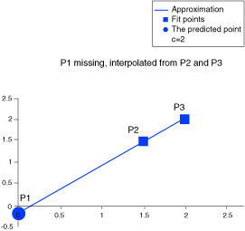
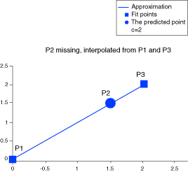
For a value $c = 1.15$ , a good approximation of a step function can be achieved with just seven interpolation points. For a value of $c = 2$ , a good approximation of a linear function can be achieved with just three interpolation points, as shown in the following figure:

For a value $c = 3$ , a good approximation of a harmonic function is achieved with about seven points per harmonic period.

Picking $c = 3$ for the step function example would produce an approximation that would go through the seven data points, but it would more resemble a single sine wave than a step function. There are obviously an infinite number of solutions that will go through any given set of data points.

In most of the literature this problem is solved by splitting the interpolation data into two groups. One group is used to create the radial basis function approximation, and one group is used to compute the error between the radial basis function approximation for those points and the actual function values. The shape function is optimized to minimize the summed errors. This is a valid approach when a lot of data points are available for the interpolation; however, typical design problems in Isight deal mostly with very sparse data sets, and it seems inefficient to use only half the data to create the actual response surface.

Isight uses a different approach. Isight defines a good fit as one whereby the shape of the curve does not change when a point is subtracted. It optimizes the value of $c$ for a minimum sum of the errors for $N - 1$ data points.

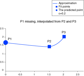
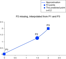
This approach can be illustrated by reviewing the graph of the straight line approximation below (P1 missing) the point P1 is approximated using the points P2 and P3; in the graph below (P2 missing) the point P2 is approximated from the two extreme points P1 and P3. For $c = 2$ , the sum of the errors for the “missing points” is low as seen in the figure.

For $c = 0.2$ , the sum of the errors of the “missing points” is extremely high.

Because the shape function optimization is given a limited number of iterations to converge, higher accuracy can be achieved by splitting up a large problem into coupled smaller ones. For example, one approximation of five inputs and two outputs and one approximation of six inputs and one output; instead of a single approximation of eleven inputs and three outputs.

Generalizing Radial Basis Functions to Elliptical Basis Functions

Radial Basis Functions can be generalized to Elliptical Basis Functions by using the Mahalanobis distance in place of the Euclidian distance in Eqn 1 and Eqn 3 (Mak and Li, 2000).

The Mahalanobis distance is defined as

{| | x - y_{j} | |}_{m}^{2} = {(x - x_{j})}_{T} S^{- 1} (x - x_{j}),

where $S$ is a symmetric positive definite matrix, also called the covariance matrix. The Euclidian distance is obtained when $S$ is taken as the identity matrix. The choice of the covariance matrix determines the quality of approximation.

To choose a good covariance matrix, Isight first assumes that the covariance of the sample data is a good approximation of the design data; i.e.,

S \approx \frac{1}{N} \sum_{i = 1}^{N} (x_{i} - μ) {(x_{i} - μ)}^{T},

where $μ$ is the centroid of the sample data. The shape function value is optimized in a manner identical to RBF.

Isight subsequently approximates the actual variance using a diagonal matrix ( $S \approx d i a g (S_{i}); i = 1, \dots, n,$ where $S_{i}$ is a positive number and $n$ is the number of input variables in the approximation). Isight optimizes the values of $S_{i}$ for a minimum sum of the errors for $N - 1$ data points using simulated annealing.

Ranking the Influence of Input Variables on Output Variables

One of the primary advantages of choosing EBF over RBF is EBF’s ability to rank the input variables in the order of influence on the output variable.

To illustrate this, consider the following example where the output $z$ depends only on one of the inputs $x$ . The values of the variable $y$ are chosen randomly.

$x$	$y$ (random)	$z$
–1	0.058834	1
–0.8	0.788471	0.894427
–0.6	0.032282	0.774587
–.4	0.916549	0.632456
–0.2	0.886644	0.447214
0	0.486239	0
0.2	0.746047	0.447214
0.4	0.804201	0.632456
0.6	0.348267	0.774597
0.8	0.441739	0.894427
1	0.733215	1

In the following figure, contour plots from both RBF and EBF approximations are shown:

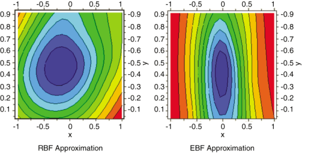
It is clear from the contour plots that EBF produces a better approximation than RBF. From the transformation matrix (see Generalizing Radial Basis Functions to Elliptical Basis Functions) it is evident that $x$ is more influential than $y$ in predicting $z$ . In the EBF model shown by the contour plots, the distance is calculated as

{‖ x - x_{j} ‖}_{m}^{2} = {(x - x_{j})}^{T} [\begin{matrix} 7.513695 & 0 \\ 0 & 0.757572 \end{matrix}] (x_{1} - x_{j})