Executing the Model and Viewing the Results

With the model open in the Design Gateway, click the button.

By default, the History tab in the Runtime Gateway opens, and the simulation code runs.

Note: If you want to change the tab that opens by default in the Runtime Gateway, see Setting Execution Preferences.

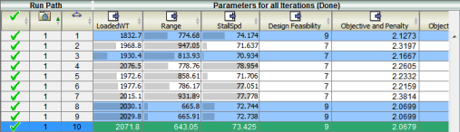
From the History tab, you can see that the ApproxLoop component obtained good solutions with respect to the objectives (minimizing the loaded weight and stall speed, and maximizing the range). Many of the bounded variables reached their lower or upper bounds, meaning that the solution has been constrained by the allowed variability of the inputs. The starting point for the analysis had the following initial values:

After the ApproxLoop component executed the simulation process flow multiple times, the best solutions were found:

The model's objective value was reduced from a starting point value of 0.780 to 0.404, which is almost a 50% improvement.

Create a history graph for the StallSpd parameter to chart the progress through the simulation process flow:

1. Click the Graphs tab.
2. Click the Graphs button.

   The Graph Chooser appears.

3. Select History Graph, and click Next.
4. Select Stallspd, and click Finish.

You can move your cursor over the points to see the different values.

Create a history graph for LoadedWT.

Create a history graph for Range.

To view all the runs, see Viewing the Benefits of the Approximation.