Rerunning the analysis with output filtering

Modifying the history output requests

When Abaqus writes nodal history output to the output database, it gives each data object a name that indicates the recorded output variable, the filter used (if any), the part instance name, the node number, and the node set. For this exercise you will be creating multiple output requests for the node in set BotChip that differ only by the output sample rate, which is not a component of the history output name. To easily distinguish between the similar output requests, create two new sets for the bottom chip reference node. Name one of the new sets BotChip-all and the other BotChip-largeInc.

Next, copy the history output request for the bottom chip three times. Edit the first copy to activate the Antialiasing filter; for this request continue to record data every 7 × 10⁻⁵ s using the set BotChip. Edit the second copy to record the data at every time increment; apply this output request to the set BotChip-all. Edit the third copy to record the data at every 7 × 10⁻⁴ s; apply this output request to the set BotChip-largeInc and activate the Antialiasing filter. When you are finished, there will be four history output requests for the bottom chip (the original one and the three added here).

Edit the output request for the strains in the set BotBoard in order to activate the Antialiasing filter.

Although we will not be discussing the results here, you may wish to add the Antialiasing filter to the history output request for the displacement, velocity, and acceleration of the node sets MidChip and TopChip.

Save your model database, and submit the job for analysis.

Evaluating the filtered acceleration of the bottom chip

When the analysis completes, test the plausibility of the acceleration history output for the bottom chip recorded every 0.07 ms using the built-in, antialiasing filter. Do this by saving and then integrating the filtered acceleration data (A3_ANTIALIASING for set BotChip) and comparing the results to recorded velocity and displacement data, just as you did earlier for the unfiltered version of these results. This time you should find that the velocity and displacement curves calculated by integrating the filtered acceleration are very similar to the velocity and displacement values written to the output database during the analysis. You may also have noticed that the velocity and displacement results are the same regardless of whether or not the built-in antialiasing filter is used. This is because the highest frequency content of the nodal velocity and displacement curves is much less than half the sampling rate. Consequently, no aliasing occurred when the data was recorded without filtering, and when the built-in antialiasing filter was applied it had no effect because there was no high frequency response to remove.

Next, compare the acceleration A3 history output recorded every increment with the two acceleration A3 history curves recorded every 0.07 ms. Plot the data recorded at every increment first so that it does not obscure the other results.

To plot the acceleration histories

In the Results Tree, filter the History Output container according to *A3*BOTCHIP* and double-click the acceleration A3 history output for the node set BotChip-all.
Select the two acceleration A3 history output objects for the node set BotChip (one filtered with the built-in antialiasing filter and the other with no filtering) using CtrlClick; click mouse button 3 and select Add to Plot from the menu that appears.

The X–Y plot appears in the viewport. Zoom in to view only the first third of the results and customize the plot appearance to obtain a plot similar to Figure 1.

Figure 1. Comparison of acceleration output with and without filtering.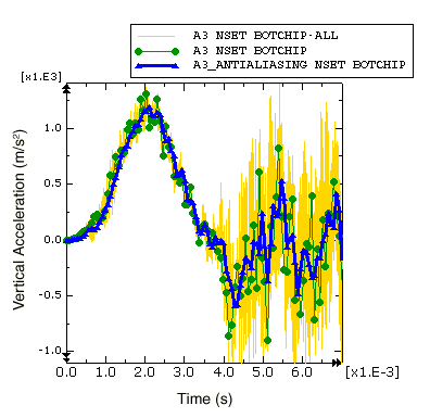

First consider the acceleration history recorded every increment. This curve contains a lot of data, including high-frequency solution noise which becomes so large in magnitude that it obscures the structurally-significant lower-frequency components of the acceleration. When output is requested every increment, the output time increment is the same as the stable time increment, which (in order to ensure stability) is based on a conservative estimate of the highest possible frequency response of the model. Frequencies of structural significance are typically two to four orders of magnitude less than the highest frequency of the model. In this example the stable time increment ranges between 8.4 × 10⁻⁴ ms to 8.8 × 10⁻⁴ ms (see the status file, Circuit.sta), which corresponds to a sample rate of about 1 MHz; this sample rate has been rounded down for this discussion, even though it means that the value is not conservative. Recalling the Sampling Theorem, the highest frequency that can be described by a given sample rate is half that rate; therefore, the highest frequency of this model is about 500 kHz and typical structural frequencies could be as high as 2–3 kHz (more than 2 orders of magnitude less than the highest model frequency). While the output recorded every increment contains a lot of undesirable solution noise in the 3 to 500 kHz range, it is guaranteed to be good (not aliased) data, which can be filtered later with a postprocessing operation if necessary.

Next consider the data recorded every 0.07 ms without any filtering. Recall that this is the curve we know to be corrupted by aliasing. The curve jumps from point to point by directly including whatever the raw acceleration value happens to be after each 0.07 ms interval. The variable nature of the high-frequency noise makes this aliased result very sensitive to otherwise imperceptible variations in the solution (due to differences between computer platforms, for example), hence the results you recorded every 0.07 increments may be significantly different from those shown in Figure 1. Similarly, the velocity and displacement curves we produced by integrating the aliased acceleration (Figure 4 and Figure 5) data are extremely sensitive to small differences in the solution noise.

When the built-in antialiasing filter is applied to the output requested every 0.07 ms, frequency content that is too high to be captured by the 14.3 kHz sample rate is filtered out before the result is written to the output database. To do this, Abaqus internally defines a low-pass, second-order, Butterworth filter. Low-pass filters attenuate the frequency content of a signal that is above a specified cutoff frequency. An ideal low-pass filter would completely eliminate all frequencies above the cutoff frequency while having no effect on the frequency content below the cutoff frequency. In reality there is a transition band of frequencies surrounding the cutoff frequency that are partially attenuated. To compensate for this, the built-in antialiasing filter has a cutoff frequency that is one-sixth of the sample rate, a value lower than the Nyquist frequency of one-half the sample rate. In most cases (including this example), this cutoff frequency is adequate to ensure that all frequency content above the Nyquist frequency has been removed before the data are written to the output database.

Abaqus/Explicit does not check to ensure that the specified output time interval provides an appropriate cutoff frequency for the internal antialiasing filter; for example, Abaqus does not check that only the noise of the signal is eliminated. When the acceleration data are recorded every 0.07 ms, the internal antialiasing filter is applied with a cutoff frequency of 2.4 kHz. This cutoff frequency is nearly the same value we previously determined to be the maximum physically meaningful frequency for the model (more than two orders of magnitude less than the maximum frequency the stable time increment can capture). The 0.07 ms output interval was intentionally chosen for this example to avoid filtering frequency content that could be physically meaningful. Next, we will study the results when the antialiasing filter is applied with a sample interval that is too large.

To plot the filtered acceleration histories

In the Results Tree, double-click the acceleration A3 history output for the node set BotChip-all.
Select the two filtered acceleration A3_ANTIALIASING history output objects for the bottom chip; click mouse button 3 and select Add to Plot from the menu that appears.

The X–Y plot appears in the viewport. Zoom out and customize the plot appearance to obtain a plot similar to Figure 2.

Figure 2. Filtered acceleration with different output sampling rates.

Figure 2 clearly illustrates some of the problems that can arise when the built-in antialiasing filter is used with too large an output time increment. First, notice that many of the oscillations in the acceleration output are filtered out when the acceleration is recorded with large time increments. In this dynamic impact problem it is likely that a significant portion of the removed frequency content is physically meaningful. Previously, we estimated that the frequency of the structural response may be as large as 2–3 kHz; however, when the sample interval is 0.7 ms, filtering is performed with a low cutoff frequency of 0.24 kHz (sample interval of 0.7 ms corresponds to a sample frequency of 1.43 kHz, one-sixth of which is the 0.24 kHz cutoff frequency). Even though the results recorded every 0.7 ms may not capture all physically meaningful frequency content, it does capture the low-frequency content of the acceleration data without distortions due to aliasing. Keep in mind that filtering decreases the peak value estimations, which is desirable if only solution noise is filtered, but can be misleading when physically meaningful solution variations have been removed.

Another issue to note is that there is a time delay in the acceleration results recorded every 0.7 ms. This time delay (or phase shift) affects all real-time filters. The filter must have some input in order to produce output; consequently the filtered result will include some time delay. While some time delay is introduced for all real-time filtering, the time delay becomes more pronounced as the filter cutoff frequency decreases; the filter must have input over a longer span of time in order to remove lower frequency content. Increasing the filter order (an option if you have created a user-defined filter, rather than using the second-order built-in antialiasing filter) also results in an increase in the output time delay. For more information, see Filtering output and operating on output in Abaqus/Explicit.

Use the real-time filtering functionality with caution. In this example we would not have been able to identify the problems with the heavily filtered data if we did not have appropriate data for comparison. In general it is best to use a minimal amount of filtering in Abaqus/Explicit, so that the output database contains a rich, un-aliased, representation for the solution recorded at a reasonable number of time points (rather than at every increment). If additional filtering is necessary, it can be done as a postprocessing operation in Abaqus/CAE.

Filtering acceleration history in Abaqus/CAE

In this section we will use the Visualization module in Abaqus/CAE to filter the acceleration history data written to the output database. Filtering as a postprocessing operation in the Visualization module has several advantages over the real-time filtering available in Abaqus/Explicit. In the Visualization module you can quickly filter X–Y data and plot the results. You can easily compare the filtered results to the unfiltered results to verify that the filter produced the desired effect. Using this technique you can quickly iterate to find appropriate filter parameters. In addition, the Visualization module filters do not suffer from the time delay that is unavoidable when filtering is applied during the analysis. Keep in mind, however, that postprocessing filters cannot compensate for poor analysis history output; if the data has been aliased or if physically meaningful frequencies have been removed, no postprocessing operation can recover the lost content.

To demonstrate the differences between filtering in the Visualization module and filtering in Abaqus/Explicit, we will filter the acceleration of the bottom chip in the Visualization module and compare the results to the filtered data Abaqus/Explicit wrote to the output database.

To filter acceleration history:

In the Results Tree, select the acceleration A3 history output for the node set BotChip-all, and save the data as A3-all.
In the Results Tree, double-click XYData; then select Operate on XY data in the Create XY Data dialog box. Click Continue.
In the Operate on XY Data dialog box, filter A3-all with filter options that are equivalent to those applied by the Abaqus/Explicit built-in antialiasing filter when the output increment is 0.7 ms. Recall that the built-in antialiasing filter is a second-order Butterworth filter with a cutoff frequency that is one-sixth of the output sample rate; hence, the expression at the top of the dialog box should appear as
```
butterworthFilter ( xyData="A3-all", 
 cutoffFrequency=1/(6*0.0007) )
```
Click Plot Expression to plot the filtered acceleration curve.
In the Results Tree, click mouse button 3 on the filtered acceleration A3_ANTIALIASING history output for node set BotChip-largeInc; and select Add to Plot from the menu that appears. If you wish, also add the filtered acceleration history for the node set BotChip.

The X–Y plot appears in the viewport. As before, customize the plot appearance to obtain a plot similar to Figure 3.

Figure 3. Comparison of acceleration filtered in Abaqus/Explicit and the Visualization module.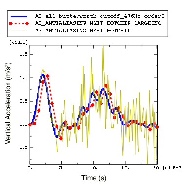

In Figure 3 it is clear that the postprocessing filter in the Visualization module of Abaqus/CAE does not suffer from the time delay that occurs when filtering is performed while the analysis is running. This is because the Visualization module filters are bidirectional, which means that the filtering is applied first in a forward pass (which introduces some time delay) and then in a backward pass (which removes the time delay). As a consequence of the bidirectional filtering in the Visualization module, the filtering is essentially applied twice, which results in additional attenuation of the filtered signal compared to the attenuation achieved with a single-pass filter. This is why the local peaks in the acceleration curve filtered in the Visualization module are a bit lower than those in the curve filtered by Abaqus/Explicit.

To develop a better understanding of the Visualization module filtering capabilities, return to the Operate on XY Data dialog box and filter the acceleration data with other filter options. For example, try different cutoff frequencies.

Can you confirm that the cutoff frequency of 2.4 kHz associated with the built-in antialiasing filter with a time increment size of 0.07 was appropriate? Does increasing the cutoff frequency to 6 kHz, 7 kHz, or even 10 kHz produce significantly different results?

You should find that a moderate increase in the cutoff frequency does not have a significant effect on the results, implying that we probably have not missed physically meaningful frequency content when we filtered with a cutoff frequency of 2.4 kHz.

Compare the results of filtering the acceleration data with Butterworth and Chebyshev Type I filters. The Chebyshev filter requires a ripple factor parameter (rippleFactor), which indicates how much oscillation you will allow in exchange for an improved filter response; see Filtering output and operating on output in Abaqus/Explicit for more information. For the Chebyshev Type I filter a ripple factor of 0.071 will result in a very flat pass band with a ripple that is only 0.5%.

You may not notice much difference between the filters when the cutoff frequency is 5 kHz, but what about when the cutoff frequency is 2 kHz? What happens when you increase the order of the Chebyshev Type I filter?

Compare your results to those shown in Figure 4.

Figure 4. Comparison of acceleration filtered with Butterworth and Chebyshev Type I filters.

Note:

The Abaqus/CAE postprocessing filters are second-order by default. To define a higher order filter you can use the filterOrder parameter with the butterworthFilter and the chebyshev1Filter operators. For example, use the following expression in the Operate on XY Data dialog box to filter A3-all with a sixth-order Chebyshev Type I filter using a cutoff frequency of 2 kHz and a ripple factor of 0.017.

chebyshev1Filter ( xyData="A3-all" , cutoffFrequency=2000,
 rippleFactor= 0.017, filterOrder=6)

The second-order Chebyshev Type I filter with a ripple factor of 0.071 is a relatively weak filter, so some of the frequency content above the 2 kHz cutoff frequency is not filtered out. When the filter order is increased, the filter response is improved so that the results are more like the equivalent Butterworth filter. For more information on the X–Y data filters available in Abaqus/CAE see Operating on saved X–Y data objects.

Filtering strain history in Abaqus/CAE

Strain in the circuit board near the location of the chips is another result that may assist us in determining the effectiveness of the foam packaging. If the strain under the chips exceeds a limiting value, the solder securing the chips to the board will fail. We wish to identify the peak strain in any direction. Therefore, the maximum and minimum principal logarithmic strains are of interest. Principal strains are one of a number of Abaqus results that are derived from nonlinear operators; in this case a nonlinear function is used to calculate principal strains from the individual strain components. Some other common results that are derived from nonlinear operators are principal stresses, Mises stress, and equivalent plastic strains. Care must be taken when filtering results that are derived from nonlinear operators, because nonlinear operators (unlike linear ones) can modify the frequency of the original result. Filtering such a result may have undesirable consequences; for example, if you remove a portion of the frequency content that was introduced by the application of the nonlinear operator, the filtered result will be a distorted representation of the derived quantity. In general, you should either avoid filtering quantities derived from nonlinear operators or filter the underlying quantities before calculating the derived quantity using the nonlinear operator.

The strain history output for this analysis was recorded every 0.07 ms using the built-in antialiasing filter. To verify that the antialiasing filter did not distort the principal strain results, we will calculate the principal logarithmic strains using the filtered strain components and compare the result to the filtered principal logarithmic strains.

To calculate the principal logarithmic strains:

To identify the elements in set BotBoard that are closest to the bottom chip (use the ODB display options to display the mass elements), plot the undeformed circuit board with element numbers visible.
In the Results Tree, filter the History Output according to *LE*Element#*, where # is the number of one of the elements in set BotBoard that is close to the bottom chip. Select the logarithmic strain component LE11 on the SPOS surface of the element, and save the data as LE11.
Similarly, save the LE12 and LE22 strain components for the same element as LE12 and LE22, respectively.
In the Results Tree, double-click XYData; then select Operate on XY data in the Create XY Data dialog box. Click Continue.
In the Operate on XY Data dialog box, use the saved logarithmic strain components to calculate the maximum principal logarithmic strain. The expression at the top of the dialog box should appear as:
```
(("LE11"+"LE22")/2) + sqrt( power(("LE11"-"LE22")/2,2)
 + power("LE12"/2,2) )
```
Click Save As to save calculated maximum principal logarithmic strain as LEP-Max.
Edit the expression in the Operate on XY Data dialog box to calculate the minimum principal logarithmic strain. The modified expression should appear as:
```
(("LE11"+"LE22")/2) - sqrt( power(("LE11"-"LE22")/2,2)
 + power("LE12"/2,2) )
```
Click Save As to save calculated minimum principal logarithmic strain as LEP-Min.

In order to plot the calculated principal logarithmic strains with the same Y-axis as the strains recorded during the analysis, change the Y-value type to strain.
In the XYData container of the Results Tree, click mouse button 3 on LEP-Max; and select Edit from the menu that appears.
In the Edit XY Data dialog box, choose Strain as the Y-value type.
Similarly, edit LEP-Min and select Strain as the Y-value type.
Using the Results Tree, plot LEP-Man and LEP-Min along with the principal strains recorded during the analysis (LEP1 and LEP2) for the same element in set BotBoard.
As before, customize the plot appearance to obtain a plot similar to Figure 5. The actual plot will depend on which element you selected.

Figure 5. Principal logarithmic strain values versus time.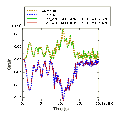

In Figure 5 we see that the filtered principal logarithmic strain curves recorded during the analysis are indistinguishable from the principal logarithmic strain curves calculated from the filtered strain components. Therefore the antialiasing filter (cutoff frequency 2.4 kHz) did not remove any of the frequency content introduced by the nonlinear operation to calculate principal strains form the original strain data. Next, filter the strain data with a lower cutoff frequency of 500 Hz.

To filter principal logarithmic strains with a cutoff frequency
of 500 Hz:

In the Results Tree, double-click XYData; then select Operate on XY data in the Create XY Data dialog box. Click Continue.
In the Operate on XY Data dialog box, filter the maximum principal logarithmic strain LEP-Max using a second-order Butterworth filter with a cutoff frequency of 500 Hz. The expression at the top of the dialog box should appear as:
```
butterworthFilter(xyData="LEP-Max", cutoffFrequency=500)
```
Click Save As to save the calculated maximum principal logarithmic strain as LEP-Max-FilterAfterCalc-bw500.
Similarly, filter the logarithmic strain components LE11, LE12, and LE22 using the same second-order Butterworth filter with a cutoff frequency of 500 Hz. Save the resulting curves as LE11–bw500, LE12–bw500, and LE22–bw500, respectively.
Now calculate the maximum principal logarithmic strain using the filtered logarithmic strain components. The expression at the top of the Operate on XY Data dialog box should appear as:
```
(("LE11-bw500"+"LE22-bw500")/2) + sqrt( 
 power(("LE11-bw500"-"LE22-bw500")/2,2) + 
 power("LE12-bw500"/2,2) )
```
Click Save As to save the calculated maximum principal logarithmic strain as LEP-Max-CalcAfterFilter-bw500.
In the XYData container of the Results Tree, click mouse button 3 on LEP-Max-CalcAfterFilter-bw500; and select Edit from the menu that appears.
In the Edit XY Data dialog box, choose Strain as the Y-value type.
Plot LEP-Max-CalcAfterFilter-bw500 and LEP-Max-FilterAfterCalc-bw500 as shown in Figure 6. As before, the actual plot will depend on which element you selected.

Figure 6. Principal logarithmic strain calculated before and after filtering (cutoff frequency 500 Hz).

In Figure 6 you can see that there is a significant difference between filtering the strain data before and after the principal strain calculation. The curve that was filtered after the principal strain calculation is distorted because some of the frequency content introduced by applying the nonlinear principal-stress operator is higher than the 500 Hz filter cutoff frequency. In general, you should avoid directly filtering quantities that have been derived from nonlinear operators; whenever possible filter the underlying components and then apply the nonlinear operator to the filtered components to calculate the desired derived quantity.

Strategy for recording and filtering Abaqus/Explicit history output

Recording output for every increment in Abaqus/Explicit generally produces much more data than you need. The real-time filtering capability allows you to request history output less frequently without distorting the results due to aliasing. However, you should ensure that your output rate and filtering choices have not removed physically meaningful frequency content nor distorted the results (for example, by introducing a large time delay or by removing frequency content introduced by nonlinear operators). Keep in mind that no amount of postprocessing filtering can recover frequency content filtered out during the analysis, nor can postprocessing filtering recover an original signal from aliased data. In addition, it may not be obvious when results have been over-filtered or aliased if additional data are not available for comparison. A good strategy is to choose a relatively high output rate and use the Abaqus/Explicit filters to prevent aliasing of the history output, so that valid and rich results are written to the output database. You may even wish to request output at every increment for a couple of critical locations. After the analysis completes, use the postprocessing tools in Abaqus/CAE to quickly and iteratively apply additional filtering as desired.